
Journal of Systems Engineering and Electronics ›› 2022, Vol. 33 ›› Issue (2): 370-380.doi: 10.23919/JSEE.2022.000039
• SYSTEMS ENGINEERING • Previous Articles Next Articles
Pingping XIONG1,*( ), Shiting CHEN2(), Shuli YAN1()
Received:2020-10-12
Online:2022-05-06
Published:2022-05-06
Contact:
Pingping XIONG
E-mail:xpp8125@163.com;1780458169@qq.com;yshuli@126.com
About author:Supported by:Pingping XIONG, Shiting CHEN, Shuli YAN. Time-delay nonlinear model based on interval grey number and its application[J]. Journal of Systems Engineering and Electronics, 2022, 33(2): 370-380.
Add to citation manager EndNote|Reference Manager|ProCite|BibTeX|RefWorks
Table 1
Average relative error and prediction accuracy of the model"
| Average relative error/% | Prediction accuracy |
| <10 | Higher |
| 10?20 | High |
| 20?50 | Medium |
| >50 | Low |
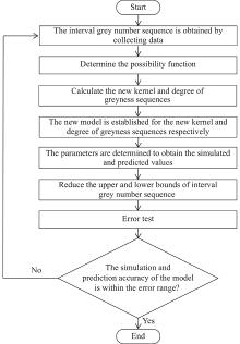
Fig 1
Modeling flow chart"
Table 2
Possibility function"
| Data | | |
| Dec.24 | | |
| Dec.25 | | |
| Dec.26 | | |
| Dec.27 | | |
| Dec.28 | | |
| Dec.29 | | |
| Dec.30 | | |
| Dec.31 | | |
| Jan.1 | | |
| Jan.2 | | |
| Jan.3 | | |
| Jan.4 | | |
| Jan.5 | | |
| Jan.6 | | |
| Jan.7 | | |
| Jan.8 | | |
| Jan.9 | | |
| Jan.10 | | |
| Jan.11 | | |
| Jan.12 | | |
| Jan.13 | | |
| Jan.14 | | |
| Jan.15 | | |
| Jan.16 | | |
| Jan.17 | | |
Table 3
Simulated and predicted values"
| Value | n | AQI | Visibility /km |
| Simulated value | 1 | [51.00,77.00] | [8.80,23.80] |
| 2 | [53.37,76.62] | [9.14,19.91] | |
| 3 | [58.28,76.75] | [8.86,16.25] | |
| 4 | [58.19,76.73] | [8.83,19.67] | |
| 5 | [57.56,76.81] | [8.90,21.89] | |
| 6 | [57.55,76.97] | [9.18,19.83] | |
| 7 | [57.03,76.63] | [10.12,20.31] | |
| 8 | [57.34,76.74] | [10.63,22.80] | |
| 9 | [59.19,83.46] | [10.63,24.06] | |
| 10 | [61.40,81.84] | [10.64,24.17] | |
| 11 | [58.00,80.94] | [10.65,18.72] | |
| 12 | [71.72,90.83] | [6.67,14.63] | |
| 13 | [73.40,91.35] | [6.66,14.65] | |
| Predicted value | 14 | [72.69,90.34] | [6.51,15.39] |
| 15 | [74.54,90.14] | [6.66,15.75] |
Table 4
Relative error"
| Erorr | | AQI | Visibility | |||
| L/% | U/% | L/% | U/% | |||
| Simulated error | 1 | 0.00 | 0.00 | 0.00 | 0.00 | |
| 2 | 0.70 | 0.50 | 3.83 | 16.34 | ||
| 3 | 0.48 | 0.32 | 0.70 | 0.29 | ||
| 4 | 0.32 | 0.35 | 0.34 | 0.64 | ||
| 5 | 0.97 | 0.25 | 1.18 | 9.55 | ||
| 6 | 0.97 | 0.04 | 4.31 | 18.05 | ||
| 7 | 0.05 | 0.49 | 6.54 | 16.09 | ||
| 8 | 0.60 | 0.34 | 0.30 | 5.80 | ||
| 9 | 3.83 | 10.26 | 0.31 | 0.59 | ||
| 10 | 7.71 | 12.00 | 0.33 | 0.12 | ||
| 11 | 1.76 | 18.25 | 0.48 | 0.44 | ||
| 12 | 1.02 | 13.49 | 1.07 | 0.45 | ||
| 13 | 3.38 | 13.00 | 0.84 | 0.34 | ||
| Average simulation error | 1.68 | 5.33 | 1.56 | 5.28 | ||
| Predicted error | 14 | 2.37 | 13.96 | 1.38 | 4.72 | |
| 15 | 4.99 | 14.15 | 0.90 | 7.15 | ||
| Average prediction error | 3.68 | 14.06 | 1.14 | 5.94 | ||
Table 5
Comparison of simulated and predicted values"
| Value | | Actual value | Model 1 | Model 2 | Model 3 | Model 4 | |||||||||
| AQI | Visibility/km | AQI | Visibility/km | AQI | Visibility/km | AQI | Visibility/km | AQI | Visibility/km | ||||||
| Simulated value | 1 | [51.00,77.00] | [8.80,23.80] | [51.85,69.77] | [9.27,23.85] | [51.00,77.00] | [8.80,23.80] | [51.00,77.00] | [8.80,23.80] | [51.00,77.00] | [8.80,23.80] | ||||
| 2 | [53.00,77.00] | [8.80,23.80] | [52.96,72.38] | [9.24,23.43] | [56.32,72.71] | [8.57,21.29] | [58.28,69.78] | [11.33,20.77] | [54.90,76.28] | [9.58,17.31] | |||||
| 3 | [58.00,77.00] | [8.80,16.30] | [54.08,75.00] | [9.21,23.00] | [55.00,75.19] | [9.25,21.42] | [59.97,74.53] | [8.87,16.19] | [58.88,76.86] | [9.08,16.14] | |||||
| 4 | [58.00,77.00] | [8.80,19.80] | [55.19,77.61] | [9.17,22.58] | [55.04,77.87] | [9.47,20.99] | [59.46,76.53] | [9.20,19.58] | [58.24,76.08] | [9.55,19.74] | |||||
| 5 | [57.00,77.00] | [8.80,24.20] | [56.31,80.23] | [9.14,22.16] | [55.70,79.42] | [9.16,21.77] | [57.94,76.28] | [11.18,19.88] | [57.93,76.69] | [9.62,23.52] | |||||
| 6 | [57.00,77.00] | [8.80,24.20] | [57.42,82.84] | [9.10,21.74] | [56.45,80.64] | [8.94,22.82] | [57.87,76.30] | [10.61,20.33] | [57.90,76.39] | [9.72,23.60] | |||||
| 7 | [57.00,77.00] | [9.50,24.20] | [58.54,85.46] | [9.07,21.31] | [57.25,82.11] | [8.95,23.56] | [57.76,76.41] | [10.73,21.36] | [57.92,76.23] | [10.33,23.84] | |||||
| 8 | [57.00,77.00] | [10.60,24.20] | [59.65,88.07] | [9.04,20.89] | [57.99,83.71] | [9.22,24.13] | [58.25,76.09] | [11.13,23.41] | [58.19,76.82] | [11.18,23.83] | |||||
| 9 | [57.00,93.00] | [10.60,24.20] | [60.77,90.69] | [9.00,20.47] | [58.63,86.42] | [9.84,23.80] | [64.56,85.55] | [11.31,23.25] | [62.17,83.24] | [11.29,23.68] | |||||
| 10 | [57.00,93.00] | [10.60,24.20] | [61.88,93.30] | [8.97,20.04] | [59.57,90.10] | [10.42,22.73] | [62.32,87.02] | [11.84,21.84] | [65.27,81.23] | [11.54,23.07] | |||||
| 11 | [57.00,99.00] | [10.60,18.80] | [63.00,95.92] | [8.93,19.62] | [61.28,94.74] | [10.54,20.84] | [65.05,89.78] | [10.83,18.71] | [66.26,79.90] | [11.28,18.80] | |||||
| 12 | [71.00,105.00] | [6.60,14.70] | [64.11,98.53] | [8.90,19.20] | [65.35,101.50] | [8.94,17.24] | [73.56,104.35] | [6.92,14.56] | [77.89,86.97] | [7.03,14.60] | |||||
| 13 | [71.00,105.00] | [6.60,14.70] | [65.23,101.15] | [8.87,18.77] | [71.43,109.59] | [5.80,12.70] | [72.37,103.77] | [7.03,12.27] | [79.09,84.06] | [7.08,14.59] | |||||
| Predicted value | 14 | [71.00,105.00] | [6.60,14.70] | [66.34,103.76] | [8.83,18.35] | [76.83,116.60] | [3.19,9.08] | [72.34,105.82] | [7.30,10.67] | [72.86,75.41] | [6.52,15.57] | ||||
| 15 | [71.00,105.00] | [6.60,14.70] | [67.46,106.38] | [8.80,17.93] | [81.58,122.74] | [1.13,6.22] | [63.96,104.16] | [7.17,9.55] | [84.75,84.78] | [9.78,15.68] | |||||
Table 6
Comparison of relative errors"
| Error | | Model 1 | Model 2 | Model 3 | Model 4 | |||||||||||||||||||
| AQI | Visibility | AQI | Visibility | AQI | Visibility | AQI | Visibility | |||||||||||||||||
| L/% | U/% | L/% | U/% | L/% | U/% | L/% | U/% | L/% | U/% | L/% | U/% | L/% | U/% | L/% | U/% | |||||||||
| Simulated error | 1 | 1.66 | 9.39 | 5.39 | 0.21 | 0.00 | 0.00 | 0.00 | 0.00 | 0.00 | 0.00 | 0.00 | 0.00 | 0.00 | 0.00 | 0.00 | 0.00 | |||||||
| 2 | 0.07 | 5.99 | 5.00 | 1.57 | 6.26 | 5.58 | 2.61 | 10.55 | 9.95 | 9.37 | 28.73 | 12.71 | 3.59 | 0.93 | 8.88 | 27.28 | ||||||||
| 3 | 6.77 | 2.60 | 4.61 | 41.13 | 5.17 | 2.34 | 5.09 | 31.43 | 3.40 | 3.20 | 0.84 | 0.65 | 1.51 | 0.19 | 3.17 | 0.97 | ||||||||
| 4 | 4.84 | 0.80 | 4.23 | 14.05 | 5.11 | 1.14 | 7.65 | 6.02 | 2.51 | 0.60 | 4.51 | 1.12 | 0.42 | 1.19 | 8.47 | 0.31 | ||||||||
| 5 | 1.22 | 4.19 | 3.84 | 8.44 | 2.29 | 3.14 | 4.09 | 10.06 | 1.65 | 0.94 | 27.05 | 17.85 | 1.63 | 0.40 | 9.29 | 2.83 | ||||||||
| 6 | 0.74 | 7.59 | 3.45 | 10.19 | 0.96 | 4.73 | 1.62 | 5.70 | 1.52 | 0.91 | 20.53 | 15.97 | 1.58 | 0.80 | 10.46 | 2.46 | ||||||||
| 7 | 2.69 | 10.99 | 4.53 | 11.93 | 0.44 | 6.64 | 5.77 | 2.63 | 1.33 | 0.77 | 12.96 | 11.74 | 1.62 | 1.00 | 8.78 | 1.50 | ||||||||
| 8 | 4.65 | 14.38 | 14.75 | 13.68 | 1.74 | 8.72 | 12.98 | 0.28 | 2.19 | 1.19 | 5.04 | 3.27 | 2.08 | 0.23 | 5.47 | 1.53 | ||||||||
| 9 | 6.61 | 2.48 | 15.08 | 15.43 | 2.86 | 7.07 | 7.14 | 1.65 | 13.25 | 8.01 | 6.70 | 3.91 | 9.07 | 10.49 | 6.47 | 2.16 | ||||||||
| 10 | 8.56 | 0.33 | 15.40 | 17.18 | 4.51 | 3.12 | 1.72 | 6.06 | 9.33 | 6.43 | 11.71 | 9.76 | 14.52 | 12.66 | 8.86 | 4.69 | ||||||||
| 11 | 10.52 | 3.11 | 15.72 | 4.36 | 7.51 | 4.31 | 0.58 | 10.83 | 14.12 | 9.32 | 2.20 | 0.47 | 16.25 | 19.29 | 6.41 | 0.02 | ||||||||
| 12 | 9.70 | 6.16 | 34.85 | 30.59 | 7.96 | 3.34 | 35.39 | 17.30 | 3.60 | 0.61 | 4.91 | 0.94 | 9.70 | 17.17 | 6.49 | 0.66 | ||||||||
| 13 | 8.13 | 3.67 | 34.33 | 27.71 | 0.61 | 4.37 | 12.19 | 13.61 | 1.92 | 1.17 | 6.47 | 16.52 | 11.39 | 19.95 | 7.31 | 0.75 | ||||||||
| Average simulation error | 5.09 | 5.51 | 12.40 | 15.11 | 3.49 | 4.19 | 7.45 | 8.93 | 4.98 | 3.27 | 10.13 | 7.30 | 5.64 | 6.48 | 6.93 | 3.47 | ||||||||
| Predicted error | 14 | 6.56 | 1.18 | 33.82 | 24.84 | 8.22 | 11.05 | 51.69 | 38.24 | 1.89 | 0.78 | 10.59 | 27.43 | 2.62 | 28.18 | 1.24 | 5.90 | |||||||
| 15 | 4.99 | 1.31 | 33.30 | 21.96 | 14.90 | 16.90 | 82.95 | 57.65 | 9.92 | 1.10 | 8.69 | 35.00 | 19.37 | 19.26 | 48.20 | 6.69 | ||||||||
| Average prediction error | 5.78 | 1.25 | 33.56 | 23.40 | 11.56 | 13.97 | 67.32 | 47.95 | 5.90 | 0.94 | 9.64 | 31.22 | 10.99 | 23.72 | 24.72 | 6.30 | ||||||||
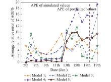
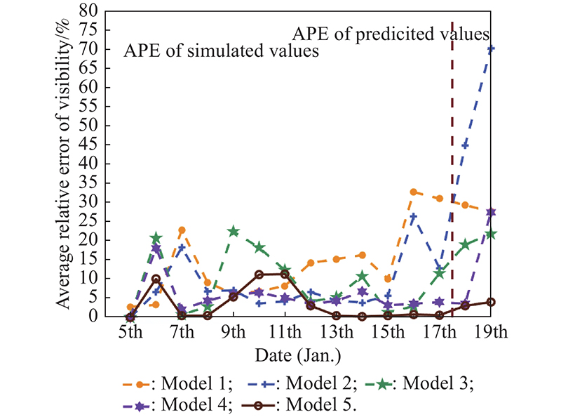
Fig 2
Comparison of average relative error of AQI "
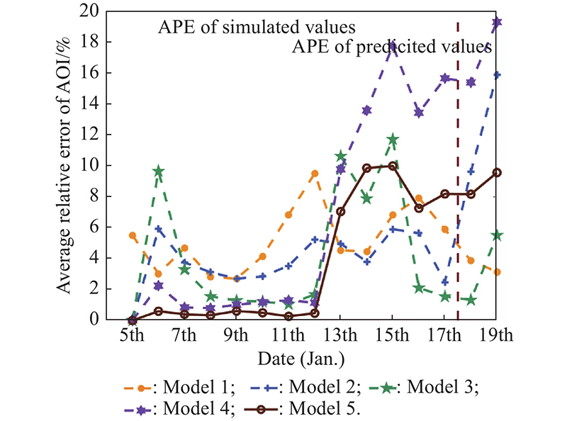
Fig 3
Comparison of average relative error of visibility "
| 1 | SUN X Z, WANG K, LI B, et al Exploring the cause of PM 2.5 pollution episodes in a cold metropolis in China. Journal of Cleaner Production, 2020, 256, 120275. |
| 2 | ZHAO Q, YUAN C H Did haze pollution harm the quality of economic development?—An empirical study based on China’s PM2.5 concentrations. Sustainability, 2020, 12 (4): 1607. |
| 3 | LEI Y H Hazards of haze and countermeasures. Applied Mechanics and Materials, 2014, 507, 817- 820. |
| 4 |
GAO L N, CAO L J, ZHANG Y, et al Re-evaluating the distribution and variation characteristics of haze in China using different distinguishing methods during recent years. Science of the Total Environment, 2020, 732, 138905.
doi: 10.1016/j.scitotenv.2020.138905 |
| 5 | WANG F C, ZHENG P, DAI J L, et al Fault tree analysis of the causes of urban smog events associated with vehicle exhaust emissions: a case study in Jinan, China. Science of the Total Environment, 2019, 668, 245- 253. |
| 6 | ZHANG J J, CHU X H, MEI T Causes of continuous haze pollution in Jiujiang City. Meteorological and Environmental Research, 2020, 11 (3): 16- 20. |
| 7 | YAN J C, LIANG X G, LIN M G, et al A hybrid features learning model for single image haze prediction. Signal, Image and Video Processing, 2018, 12 (11): 1- 8. |
| 8 |
YIN Z C, WANG H J Statistical prediction of winter haze days in the north China plain using the generalized additive model. Journal of Applied Meteorology and Climatology, 2017, 56 (9): 2411- 2419.
doi: 10.1175/JAMC-D-17-0013.1 |
| 9 |
SHAWKI D, FIELD R D, TIPPETT M K, et al Long-lead prediction of the 2015 fire and haze episode in Indonesia. Geophysical Research Letters, 2017, 44 (19): 9996- 10005.
doi: 10.1002/2017GL073660 |
| 10 |
ZHANG M, LIU X X, DING Y T, et al How does environmental regulation affect haze pollution governance?—An empirical test based on Chinese provincial panel data. Science of the Total Environment, 2019, 695, 133905.
doi: 10.1016/j.scitotenv.2019.133905 |
| 11 |
ZHANG M, LI H, XUE L Z, et al Using three-sided dynamic game model to study regional cooperative governance of haze pollution in China from a government heterogeneity perspective. Science of the Total Environment, 2019, 694, 133559.
doi: 10.1016/j.scitotenv.2019.07.365 |
| 12 |
LI H, ZHANG M, LI C, et al Study on the spatial correlation structure and synergistic governance development of the haze emission in China. Environmental Science and Pollution Research International, 2019, 26 (12): 12136- 12149.
doi: 10.1007/s11356-019-04682-5 |
| 13 | KONG Y W, SHENG L F, LI Y P, et al Improving PM2. 5 forecast during haze episodes over China based on a coupled 4D-LETKF and WRF-Chem system. Atmospheric Research, 2021, 249, 105366. |
| 14 |
ZHANG M D, YANG J W, ZHANG W M, et al Analysis, prediction and application of Beijing smog based on ARIMA. Statistics and Application, 2019, 8 (2): 381- 393.
doi: 10.12677/SA.2019.82043 |
| 15 | LIU D Y, HE Y D, WANG Q R Urban spatial structure evolution and smog management in China: a re-examination using nonparametric panel model. Journal of Cleaner Production, 2020, 285, 124847. |
| 16 |
FU B, GAO X H, WU L F Grey relational analysis for the AQI of Beijing, Tianjin, and Shijiazhuang and related countermeasures. Grey Systems-Theory and Application, 2018, 8 (2): 156- 166.
doi: 10.1108/GS-12-2017-0046 |
| 17 | ZHANG R H, SUN B, LIU M Y, et al Haze pollution, new-type urbanization and regional total factor productivity growth: based on a panel dataset involving all 31 provinces within the territory of China. Kybernetes, 2020, 50 (5): 1357- 1378. |
| 18 | LI S L, ZENG B, MA X, et al A novel grey model with a three-parameter background value and its application in forecasting average annual water consumption per capita in urban areas along the Yangtze River Basin. Journal of Grey System, 2020, 32 (1): 118- 132. |
| 19 |
KARIMI T, HOJATI A Designing a medical rule model system by using rough–grey modeling. Grey Systems: Theory and Application, 2020, 10 (4): 513- 527.
doi: 10.1108/GS-02-2020-0017 |
| 20 |
DING S, XU N, YE J, et al Estimating Chinese energy-related CO2 emissions by employing a novel discrete grey prediction model . Journal of Cleaner Production, 2020, 259, 120793.
doi: 10.1016/j.jclepro.2020.120793 |
| 21 |
DUAN J L, JIAO F, ZHANG Q S An improvement of GM (1, N) model based on support vector machine regression with nonlinear cross effects . Symmetry, 2019, 11 (5): 604.
doi: 10.3390/sym11050604 |
| 22 |
XIE W L, LIU C, WU W Z The fractional non-equidistant grey opposite-direction model with time-varying characteristics. Soft Computing, 2020, 24, 6603- 6612.
doi: 10.1007/s00500-020-04799-7 |
| 23 | ZHAI J, SHENH J M, FENG Y J The grey model MGM(1, n) and its application . Systems Engineering: Theory and Practice, 1997, 17 (5): 109- 113. |
| 24 | YUAN Z H, GUO F, QI X X Fault prediction methods study of machinery based on optimized background value MGM(1, m) model . Applied Mechanics and Materials, 2014, 3360, 1513- 1516. |
| 25 |
GE P F Application of optimization algorithm for unequal time interval MGM (1, N) in engineering survey . Geomatics Science and Technology, 2020, 8 (2): 68- 77.
doi: 10.12677/GST.2020.82009 |
| 26 | XIONG P P, HE Z Q, CHEN S T, et al A novel GM(1, N) model based on interval gray number and its application to research on smog pollution . Kybernetes, 2020, 49 (3): 753- 778. |
| 27 | XIONG P P, HUANG S, PENG M, et al. Examination and prediction of fog and haze pollution using a multi-variable grey model based on interval number sequences. Applied Mathematical Modelling, 2020, 77(Part 2): 1531−1544. |
| 28 | ZHANG F, TAN S W, ZHANG L L, et al. Fault tree interval analysis of complex systems based on universal grey operation. Complexity, 2019. DOI: 10.1155/2019/1046054. |
| 29 |
ZENG B, LI C, CHEN G, et al Verhulst model of interval grey number based on information decomposing and model combination. Journal of Applied Mathematics, 2013, 2013, (6): 1- 8.
doi: 10.1155/2013/472065 |
| 30 | ZHAO L M, ZENG B Prediction modeling method of interval grey number based on different type whitenization weight functions. Applied Mechanics and Materials, 2013, 411, 2074- 2080. |
| 31 |
LI Y, GUO S D, LI J Prediction model of three-parameter interval grey number based on kernel and double information domains. Grey Systems−Theory and Application, 2020, 10 (4): 455- 465.
doi: 10.1108/GS-09-2019-0030 |
| 32 |
MA X, MEI X, WU W Q, et al A novel fractional time delayed grey model with Grey Wolf Optimizer and its applications in forecasting the natural gas and coal consumption in Chongqing China. Energy, 2019, 178, 487- 507.
doi: 10.1016/j.energy.2019.04.096 |
| 33 |
LIU P L Stability of continuous and discrete time-delay grey systems. International Journal of Systems Science, 2001, 32 (7): 947- 952.
doi: 10.1080/00207720010005636 |
| 34 | SAHIN U Future of renewable energy consumption in France, Germany, Italy, Spain, Turkey and UK by 2030 using optimized fractional nonlinear grey Bernoulli model. Sustainable Production and Consumption, 2021, 25 (1): 1- 14. |
| 35 |
YUAN Y B, LI Q, YUAN X H, et al A SAFSA- and metabolism-based nonlinear grey Bernoulli model for annual water consumption prediction. Iranian Journal of Science and Technology, 2020, 44 (1): 1- 11.
doi: 10.1007/s40995-019-00800-7 |
| 36 | XIE M, WU L F, LI B, et al A novel hybrid multivariate nonlinear grey model for forecasting the traffic-related emissions. Applied Mathematical Modelling, 2020, 77 (2): 1242- 1254. |
| 37 |
ZHENG C L, WU W Z, XIE W L, et al Forecasting the hydroelectricity consumption of China by using a novel unbiased nonlinear grey Bernoulli model. Journal of Cleaner Production, 2021, 278, 123903.
doi: 10.1016/j.jclepro.2020.123903 |
| 38 | FU Z H, ZHENG R J Time-delay multivariable GM(1, N) coordination degree model and its application . Statistics and Decision, 2018, 34 (13): 77- 80. |
| 39 | CAI G Q, AN T Y, ZHOU S Q Grey series time-delay predicting model in state estimation for power distribution networks. Journal of Harbin Institute of Technology, 2003, 41 (2): 120- 123. |
| 40 | LI M X, LIAO R Q, DONG Y Adaptive determination of time delay in grey prediction model with time delay. IIETA, 2019, 24 (5): 519- 524. |
| 41 | ZHOU K Gray nonlinear water environment management model and its application based on genetic algorithm solution. Yangtze River, 2019, 50 (5): 20- 24, 40. |
| 42 | GUO X J, LIU S F, YANG Y J A prediction method for plasma concentration by using a nonlinear grey Bernoulli combined model based on a self-memory algorithm. Computers in Biology and Medicine, 2018, 105, 81- 91. |
| 43 | SHU H, WANG W P, XIONG P P Kernel and greyness of interval grey number under known whitening weight function. Control and Decision, 2017, 32 (12): 2190- 2194. |
| 44 | XIONG P P, ZHANG Y, XING Z, et al Multivariable time-delay discrete MGM(1, m, τ) model and its application . Statistics and Decision, 2019, 35 (8): 18- 22. |
| 45 | FAN X S, XIAO X P. Method to find τ, r in GM(1, 1| τ, r) and its application. Journal of Wuhan University of Technology (Information and Management Engineering), 2013, 35(4): 536−539. (in Chinese) |
| 46 | LEWIS C D. Industrial and business forecasting method. London: Butter-worth-Heinemann, 1982. |
| [1] | ZHANG Ao, Zhihua WANG, Qiong WU, Chengrui LIU. Generalized degradation reliability model considering phase transition [J]. Journal of Systems Engineering and Electronics, 2022, 33(3): 748-758. |
| [2] | Xinjian MA, Shiqian LIU, Huihui CHENG. Civil aircraft fault tolerant attitude tracking based on extended state observers and nonlinear dynamic inversion [J]. Journal of Systems Engineering and Electronics, 2022, 33(1): 180-187. |
| [3] | Hui WAN, Xiaohui QI, Jie LI. Stability analysis of linear/nonlinear switching active disturbance rejection control based MIMO continuous systems [J]. Journal of Systems Engineering and Electronics, 2021, 32(4): 956-970. |
| [4] | Yanan DU, Hongyuan GAO, Menghan CHEN. Direction of arrival estimation method based on quantum electromagnetic field optimization in the impulse noise [J]. Journal of Systems Engineering and Electronics, 2021, 32(3): 527-537. |
| [5] | Abdollah AZIZI, Mehdi FOROUZANFAR. Stabilizing controller design for nonlinear fractional order systems with time varying delays [J]. Journal of Systems Engineering and Electronics, 2021, 32(3): 681-689. |
| [6] | Zongxing LI, Rui ZHANG. Time-varying sliding mode control of missile based on suboptimal method [J]. Journal of Systems Engineering and Electronics, 2021, 32(3): 700-710. |
| [7] | Hongwei WANG, Penglong FENG. Fuzzy modeling of multirate sampled nonlinear systems based on multi-model method [J]. Journal of Systems Engineering and Electronics, 2020, 31(4): 761-769. |
| [8] | Yang ZHAO, Lili DONG. Adaptive back-stepping control on container ships for path following [J]. Journal of Systems Engineering and Electronics, 2020, 31(4): 780-791. |
| [9] | Lixiong LIN, Qing WANG, Bingwei HE, Xiafu PENG. Evaluation of fault diagnosability for nonlinear uncertain systems with multiple faults occurring simultaneously [J]. Journal of Systems Engineering and Electronics, 2020, 31(3): 634-646. |
| [10] | Zezhou WANG, Yunxiang CHEN, Zhongyi CAI, Yangjun GAO, Lili WANG. Methods for predicting the remaining useful life of equipment in consideration of the random failure threshold [J]. Journal of Systems Engineering and Electronics, 2020, 31(2): 415-431. |
| [11] | Hongwei WANG, Yuxiao CHEN. Parameter estimation for dual-rate sampled Hammerstein systems with dead-zone nonlinearity [J]. Journal of Systems Engineering and Electronics, 2020, 31(1): 185-193. |
| [12] | Zhongyi CAI, Zezhou WANG, Yunxiang CHEN, Jiansheng GUO, Huachun XIANG. Remaining useful lifetime prediction for equipment based on nonlinear implicit degradation modeling [J]. Journal of Systems Engineering and Electronics, 2020, 31(1): 194-205. |
| [13] | Yunfei JIA, Zhiquan ZHOU, Renbiao WU. A workload-based nonlinear approach for predicting available computing resources [J]. Journal of Systems Engineering and Electronics, 2020, 31(1): 224-230. |
| [14] | Vedadi Moghaddam TAHMINEH, Yadavar Nikravesh SEYYED KAMALEDDIN, Azam Khosravi MOHAMMAD. Constrained sliding mode control of nonlinear fractional order input affine systems [J]. Journal of Systems Engineering and Electronics, 2019, 30(5): 995-1006. |
| [15] | Xiaotian WANG, Kai ZHANG, Jie YAN. Complexity estimation of image sequence for automatic target track [J]. Journal of Systems Engineering and Electronics, 2019, 30(4): 672-683. |
| Viewed | ||||||
|
Full text |
|
|||||
|
Abstract |
|
|||||